Learn How to Create a Stacked Waterfall Chart in Excel with Decreasing Values
(Step-by-Step Tutorial)

Introduction
Waterfall charts are an essential and highly effective tool in the finance world. Their primary purpose is to display a running total, with values added or subtracted, visually illustrating how an end value is derived from an initial one.
Waterfall charts have been available in Microsoft Excel since Excel 2016, making life significantly easier for finance professionals worldwide. Before that, users had to rely on complex workarounds to build them manually. However, one subtype is still missing from Excel’s default chart options: the Stacked Waterfall Chart.
Stacked waterfall charts extend the functionality of standard waterfall charts by allowing users to see how an initial value (or multiple values) is affected by multiple categories or data sets. This can be incredibly useful when visualizing Financial Statements, Project Budget Analysis, Sales Performance, Cost Savings, Headcount Changes, and more.
Although stacked waterfall charts are not included in Excel’s standard chart library, there is fortunately a wealth of information online on how to build one from scratch. However, one crucial aspect is often overlooked: how to create a stacked waterfall chart in Excel that accurately displays decreasing or negative changes and values. Without this capability, the chart can quickly become ineffective in many real-world scenarios.
That’s why we created this tutorial - to help users build a dynamic stacked waterfall chart in Excel that handles decreasing values with ease. Built entirely with standard Excel features, every element is fully customizable and updates automatically with your data. The chart can be easily shared with other Excel users and integrates seamlessly into PowerPoint for impactful presentations, without relying on third-party tools. All you need is Excel 2013 or newer and a bit of time.
Please note: If you're looking to create a stacked waterfall chart and don't need to visualize decreasing or negative values, there's a much easier and more straightforward approach available. We recommend checking out one of the existing tutorials online and continuing with this guide only if you specifically need a stacked waterfall chart that supports decreasing values.
A quick disclaimer: creating a chart like this involves multiple steps. You’ll need to separate positive and negative variances and incorporate dummy values. Additional chart elements like stack sub-totals and connector lines introduce further complexity. So, before we dive in, here’s a friendly reminder: you can create a stacked waterfall chart like the one in this tutorial in just seconds using our Excel add-in, Pine BI!

That being said, let’s dive in!
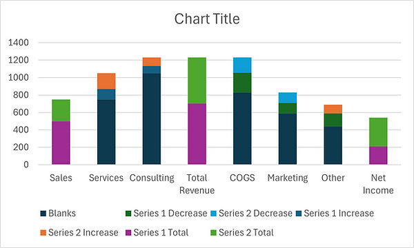
Creating the Chart
The chart we’re about to create is the same one shown at the beginning of the page. As you’ll see, we won’t just build a stacked waterfall chart with decreasing values - we’ll also incorporate additional elements and annotations such as stack sub-totals, connector lines, and rolling sub-totals. These enhancements make the chart easier to read and significantly more engaging and impactful.
While this method supports visualizing multiple data series, we’ll keep things simple by using just two data series in our example.
1. Adding Data
We'll base our chart on a simple example: a Profit and Loss statement. In this dataset, the main revenue comes from the sales of two products - Product 1 and Product 2, along with additional revenue from services and consulting related to them.
-
Row 5 shows the total revenue for each category and product.
-
Next, we have Cost of Goods Sold (COGS) and Marketing Costs, both represented as negative values.
-
The final category is Other Costs & Rebates, which includes a negative value for Product 1 and a positive value for Product 2. This could reflect rebates or promotional incentives that contribute to overall profit outside of direct revenue, but more importantly it allows us to demonstrate how the chart will handle both increasing and decreasing values in the same category.
-
The last row calculates Net Income for both product categories. It sums the revenue from sales, services, and consulting, then subtracts the associated costs.
Now that we understand the structure of our data, we’re ready to move on to building the chart itself.

2. Adding a Total Column
The first calculated column we'll add is used to indicate whether a row represents a total. Rows marked as Total will display their values in the chart with columns starting directly from the X-axis (horizontal axis). All other rows will appear as floating columns, showing the change in value relative to the previous point.
Although Sales isn’t technically a total, we’ll still mark it as one since it serves as our starting point in the chart.
-
Name this column Total.
-
For each row, enter Yes or No depending on whether it should be treated as a total.
In our case, we’ll mark Sales, Total Revenue, and Net Income as totals.

3. Adding Series Increase Calculations
Now we’ll begin adding the calculations that make the chart work.
We'll start by creating formulas that show values only if they are positive - this helps highlight increases in each product or category. Since we’re working with two data series, we’ll need to add two new columns. If you had five series, you’d need five columns - so you can see how quickly this can get complex. If you frequently work with waterfall charts or similar setups, you might want to explore the Pine BI Excel add-in, which can help automate these steps.
Create the first increase column:
-
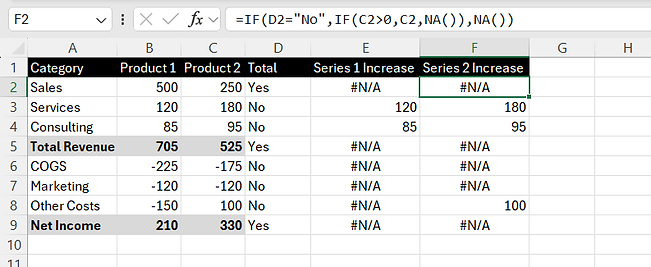
In cell E1, write the name of the column: Series 1 Increase
-
In cell E2, enter the following formula:
=IF(D2="No",IF(B2>0,B2,NA()),NA())
-
Drag the formula down to fill the column.

Create the second increase column:
-
In cell F1, write the name of the column: Series 2 Increase
-
In cell F2, enter:
=IF(D2="No",IF(C2>0,C2,NA()),NA())
-
Again, drag the formula down to apply it to all rows.
Formula Logic:
-
Check if the row is not a Total (D2="No").
-
If true, return the value only if it’s positive.
-
If the value is zero or negative, or if the row is a Total, return #N/A.
Your worksheet should now include two new columns that isolate positive changes for each series - these will be used to build the floating bars in your chart.
4. Adding Series Decrease Calculations
Just like in the previous step, we now need to create calculations for each series that isolate negative values, as these will represent the decreasing elements in the waterfall chart.
Create the first decrease column:
-
In cell G1, write the name of the column: Series 1 Decrease
-
In cell G2, enter:
=IF(D2="No",IF(B2<0,ABS(B2),NA()),NA()) -
Then drag the formula down to fill the column.
Create the second decrease column:
-
In cell H1, write the name of the column: Series 2 Decrease
-
In cell H2, enter:
=IF(D2="No",IF(C2<0,ABS(C2),NA()),NA()) -
Again, drag the formula down to apply it to all rows.
Key Differences from the Previous Step (Increase Series):
-
We're now checking if the value is less than zero (<0).
-
If it is, we return the absolute value using ABS(). This ensures the chart displays the correct column height, even though the original value is negative.
-
If the row is marked as a Total, or the value is not negative, the formula returns #N/A.
Your worksheet should now include two additional columns that capture decreases in each series. These will be used to build the downward steps in your waterfall chart.

5. Adding Series Total Calculations
Now that we've handled both positive and negative values, it's time to calculate the Totals for each series. These totals will allow the waterfall chart to dynamically reflect summary rows whenever the Total indicator in column D is set to "Yes". This setup ensures the chart remains flexible - automatically updating if rows are added, removed, or modified.
Create the first total column:
-
In cell I1, write the name of the column: Series 1 Total
-
In cell I2, add the following formula and expand down:
=IF(D2="Yes",$B$2+SUMIF($D$2:D2,"No",$B$2:B2),NA())
Formula Logic:
-
Checks if the current row is marked as a Total (D2="Yes").
-
If true:
-
Adds the starting value $B$2 (fixed for all rows).
-
Sums all non-total values from the beginning up to the current row using SUMIF($D$2:D2,"No",$B$2:B2)
-
-
If false:
-
Returns #N/A to exclude the cell from the chart.
-
-
The use of absolute references ($B$2) ensures the formula always starts from the first value in the series, even when dragged down.
Create the second total column:
-
In cell J1, write the name of the column: Series 2 Total
-
In cell J2, add the following formula and expand down:
=IF(D2="Yes",$C$2+SUMIF($D$2:D2,"No",$C$2:C2),NA())
-
This follows the same logic, but applies to the second series in column C.
Your worksheet should now include two new columns that calculate totals for each series - ready to be visualized in your waterfall chart.

6. Adding Blank Data
The Blank Values series will be used for the transparent pieces of the stacked columns, on top of which the actual series will be visualized. This is the most complex formula, as it has multiple dependencies.
-
In cell K2 write the name of the column: Blanks
-
Add the following formula in cell K2 and expand down:
=IF(D2="No",SUM($B$2:$C$2)+SUMIF($D$2:D2,"No",$B$2:B2)+SUMIF($D$2:D2,"No",$C$2:C2)-SUM(B2:C2)-ABS(SUMIF(B2:C2,"<0")),NA())
Formula Logic:
-
First, the formula checks whether this row is a Total or not. If it is a Total, it returns NA() so the column starts from the axis.
-
If it is not a Total, the following calculations take place:
-
The first row values for all products are summed. The range is fixed so the first row is added to all cells when expanding the formula: SUM($B$2:$C$2)
-
Add a sum element similar to the one used in the Total formula: sum all values between the first cell and the respective row, if they are not a Total: SUMIF($D$2:D2,"No",$B$2:B2)
-
Repeat this for the second product: SUMIF($D$2:D2,"No",$C$2:C2)
-
Subtract the product values for the respective row: SUM(B2:C2) - this ensures space for the positive or negative series columns
-
Subtract the absolute value of the sum of the product values for the respective row, only if they are negative: ABS(SUMIF(B2:C2,"<0"))
-
If the respective Total value is "Yes", the formula shows NA()
-
-
Notice how the first part of most SUM and SUMIF ranges is fixed with dollar signs.
A complicated formula indeed, but thankfully, you only need to add it once. Your data should now look like this:

For More Than 2 Products
If you need to create a stacked waterfall chart for more than 2 Products, you’ll need to expand this formula. For example, if you want to create a chart with 3 Products (values in columns B, C, and D), make the following changes:
-
The Total column with Yes/No will be pushed to column E, as column D now holds the values for Product 3
-
Change SUM($B$2:$C$2) to SUM($B$2:$D$2)
-
Add an additional SUMIF: SUMIF($E$2:E2,"No",$D$2:D2)
-
Change SUM(B2:C2) to SUM(B2:D2)
-
Change ABS(SUMIF(B2:C2,"<0")) to ABS(SUMIF(B2:D2,"<0"))
This makes the full formula for the first data row look like:
=IF(D2="No",SUM($B$2:$D$2)+SUMIF($E$2:E2,"No",$B$2:B2)+SUMIF($E$2:E2,"No",$C$2:C2)+ SUMIF($E$2:E2,"No",$D$2:D2)-SUM(B2:D2)-ABS(SUMIF(B2:D2,"<0")),NA())
Optional Simpler Formula
If you find the above formula too complex, there is a simpler alternative. The downside is that it requires the Total rows to be empty (except for the first one). The calculations also refer to the headers of the columns, which allows a single formula to be used throughout the column.
So, if you prefer, enter this formula in K2:
=IF(D2="No",SUM($B$1:C1)-ABS(SUMIF(B2:C2,"<0")),NA())
Make sure to delete the totals for Product 1 and Product 2, as shown in the print screen below - this won’t affect the other formulas.

7. Building the Chart
We now have the main calculations done and can start building our chart!
-
Select all the series calculations we've added, including their headers: E1:K9
-
Go to Insert > Charts > Insert > 2D Stacked Column Chart

This should create a chart like this:

If your chart looks different and the legend shows Series 1, Series 2, Series 3, etc., instead of the column names, go to Chart Design and select Switch Row/Column:

3. You’ll notice the data series might appear disorganized. To properly arrange the chart elements:
-
Select the chart
-
Go to Chart Design > Select Data
-
Use the arrows on the left side of the window to reorder the series:
-
Series Blank at the top
-
Followed by the Decrease Series in their respective order
-
Then the Increase Series in their respective order
-
Finally, the Totals in their respective order
-

4. While still in this menu, let’s fix the horizontal axis labels:
-
Select Series Blank
-
On the right side of the window, click Edit
-
Set the Axis label range values to A2:A9, then click OK
-
Click OK again to close the Select Data Source window

You now have a fully functional Stacked Waterfall Chart in Excel, like the one below, that supports decreasing or negative values - even if it doesn’t quite look like it yet!
All that’s left is a bit of formatting to bring it to life visually.
7. Formatting
With the hard part over, we can now finalize our visualization with the right colors. One of the advantages of the approach we're using is the flexibility it offers in coloring, allowing us to create the desired visual effect. Since the Total, Increasing, and Decreasing values are separate series, we can color them differently - whether using diverging colors or grouping them by total increase/decrease.
So, let’s get to formatting:
-
Select the Blank Data series
-
Remove the fill color:
-
Option 1 (Steps shown below in red): Go to Format > Shape Fill > No Fill
-
Option 2 (Steps shown below in amber):
-
Right-click on one of the Blank series columns > Select Format Data Series… to the Format Data Series pane on the right
-
Go to Fill & Line > Fill > No Fill
-
This will make the Blank series transparent and create the effect that the rest of the series are floating.

Next, we need to format the rest of the series:
-
Just like we did with the Blank series, select Series 1 Total, go to Format > Shape Fill, and choose the desired color.
-
Repeat this for all series to complete the chart.
You may want to format the Decreasing values differently to help distinguish them visually. This isn’t strictly necessary, but it can enhance readability. There are several ways to do this:
-
Use different colors
-
Add a border to the columns
-
Make them semi-transparent
-
Apply a pattern fill
In our example:
-
The two Total series will be colored in amber and blue for easy differentiation
-
The Increasing and Decreasing values will use pale shades of their respective totals
-
The Decreasing values will also have a red border to clearly indicate they represent a drop

8. Adding Data Labels
We now have a great Stacked Waterfall Chart, but one key element is still missing - data labels.
To add the data labels:
-
Select the chart
-
Go to Chart Elements (the plus icon next to the chart)
-
Open the Data Labels menu and choose Center

This will add data labels to all series. However, we still need to refine them to ensure they display correctly.
Step 1: Remove Data Labels from the Blank Series
Click on any data label from the Blank series and press DELETE. This will clean up the chart and remove unnecessary clutter.
Step 2: Fix Positive Labels on Decreasing Values
You may notice that the decreasing values are labeled as positive. To display them correctly as negative values:
-
Select one of the incorrect data labels for Product 1 (in orange)
-
Right-click and choose Format Data Labels (if format pane on the right not already opened)
-
The Format Data Series pane will open on the right
-
Go to Label Options
-
Select Values From Cells
-
In the pop-up window, select the actual data range (e.g., B2:B9 for Series 1) and click OK
-
The chart will now display the correct negative values from your dataset
-
Under Label options again, deselect Value, to remove the default labels
Repeat this process for all series where negative values are shown incorrectly. In our case, for Product 2.

Once complete, your chart should now display accurate and clean data labels, enhancing readability and making the visualization more intuitive.

9. Finalizing the Legend
Finally, we need to take care of the legend. Excel isn’t particularly flexible when it comes to chart legends, so depending on your needs, there may be limitations.
However, if each data series is colored differently, we can still create a clean and meaningful legend:
-
Select the chart legend
-
Select each legend entry one by one and press DELETE on your keyboard, except for Series Totals. This leaves only the Total series, which we will now rename.
Two Options for Renaming
-
Option A: Simply rename the text in cells I1 and J1 to your desired legend labels. Since these are the names of the Total series, the names will be changed in the legend as well.
-
Option B: If you want or need to keep the table header values unchanged (e.g., if your data is formatted as a table and duplicate headers aren’t allowed):
-
Select the chart
-
Go to Chart Design > Select Data
-
On the left side, select the first Total data series and click Edit

3. In the Series Name field, either:
-
Select a different cell (e.g., B1), or
-
Type a custom name manually
4. Repeat this process for all Total series

We’ve chosen to keep only the Total series in the legend, as each product typically has a total - even if some don’t have increasing or decreasing values. This can of course vary depending on your dataset.
Congratulations!
You now have a fully functional Stacked Waterfall Chart in Excel that supports negative values - ready to use in both Excel and PowerPoint.

Note: This method also works, if you want to create a Bar (vertical) chart. Just select 2D Stacked Bar Chart, instead of 2D Stacked Column Chart, when inserting the visualization at step 7. Building the Chart. However, please bare in mind that the two next optional sections - Column Sub-Totals and Connector Lines are supported only for Column (horizontal) charts with the described methodology.

Our chart looks great, but of course, we can always take it one step further by adding additional elements to help communicate the information more effectively.
Let’s see how we can add these elements.
Optional: Column Sub-Totals
Adding a sub-total for each stacked column can be very helpful in understanding how the chart evolves with each column.
The easiest way to set this up is to show all sub-totals above each column. However, since some columns may display a net negative of all changes (the total value of the sub-total may be negative, as COGS and Marketing costs in our example), we have the opportunity to make the chart easier to read by positioning the sub-total labels below those net-negative columns.
Let’s start with the simpler approach and place all sub-totals above the columns.
Note that the next steps are necessary, even if you prefer to jump straight to the more advanced sub-total data labels with the negative ones displayed under the stacks.
We'll start by adding three new columns to our table.
Create the first column:
-
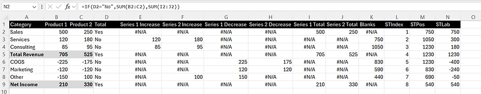
In cell L1, write the name of the column: STIndex (short for Sub-Total Index)
-
Starting with 1 in cell L2, add a consecutive number for each row. This will be used to indicate the horizontal position of the data label.

Create the second column:
-
In cell M1, write the name of the column: STPos (Sub-Total Position)
-
Enter the following formula In cell M2, which will be used to position the data labels vertically:
=SUMIF(E2:K2,">0")
-
This formula sums all positive values across the calculated columns for the respective row. It also makes the SUM() formula work, even though there are #N/A errors in the range.

Create the third column:
-
In cell N1, write the name of the column: STLab (Sub-Total Label)
-
Add the following formula in cell N2:
=IF(D2="No",SUM(B2:C2),SUM(I2:J2))
Adding the data labels
-
Select the chart, then go to Chart Design > Select Data
-
On the left side, click Add to insert a new data series.

3. For Series Name, enter: ST Label
4. For Series Values, select the range in STIndex: (L2:L9)
This will add a new data series with labels at the top of each column. But we still need to configure it properly.
Adjusting the Chart Type
-
Select the chart, then go to Chart Design > Change Chart Type
-
In the list to the left select the last option - Combo
-
Set Clustered Column for all series (some may be auto-adjusted), except for the new one STLabel - set that to Scatter
-
Ensure Secondary Axis is unchecked for all series

Configuring the New Series
-
Go back to Chart Design > Select Data window
-
Select the new data series (ST Label) and click Edit

3. The X Values may be blank - set them to the values in STIndex: L2:L9
4. For Y Values, select the values in STPos: M2:M9
Note: if you get an error when selecting the ranges for the X and Y values, you may need to first delete the old specified range.
Final Touches
Adjust the new data series to hide the markers, but show the data labels:
-
Add Data Labels
-
Click on one of the scatter markers
-
Go to Chart Elements > Data Labels > Above

2. Customize the Labels
-
Right-click one of the newly created sub-total data labels
-
Select Format Data Labels…
-
Choose Value From Cells
-
In the new window, select the values from column STLab: N2:N9
-
Deselect Y Value

3. Hide the Scatter Markers
-
Click once on one of the scatter markers to select all of them (if you click twice, only a single marker will be selected)
-
Remove the markers fill color by going to Format > Shape Fill > No Fill
-
Also remove the markers outline: Shape Outline > No Outline

At this point your chart should look like this:

If this format of the sub-total data labels works for you, just make sure to remove the unnecessary labels in the legend and you'll be ready to go! Or you can jump ahead to the optional connector lines.
However, what if we want to show the net-negative sub-totals below the stack?
Basically we need the same setup as before, but with an additional column and a slightly adjusted formula for the Labels positions.
We will use the already created structure and build upon it.
-
Leave the STIndex column as before (Starting with 1 in cell L2, add a consecutive number of each row)
-
Change the formula for STPos with the following formula in M2 and expand:
=IF(SUM(B2:C2)>=0,SUMIF(E2:K2,">0"),NA())

-
This will ensure a value is displayed only if the net total amount for the stack is positive or zero.
3. Move the STLab column to the right in column O for structural clarity (you can skip this if preferred)
4. In N2, add the name of a new column called STNeg
5. Then, add the following formula in cell N2:
=IF(SUM(B2:C2)<0,K2,NA())
-
This will handle the values for the net-negative stacks.

In the chart you will now notice that #N/A errors have appeared in column STPos, and the sub-total data labels for COGS, Marketing, and Other are now gone. They will be displayed again via a new data series, which will handle the negative values only.
We now need to add the series for the negative values.
-
Select the chart, then go to Chart Design > Select Data > Add
-
If the new window shows options for both X Values and Y Values, Excel has automatically suggested that the new data series is a scatter plot - just like the last one, which is great, as it saves time adjusting the chart. In that case, please continue with Step 2.
-
If not, you’ll need to repeat steps 1 to 4 from the previous section Adjusting the Chart Type to add the new data series and format it accordingly (for Series values select the values in range STIndex (L2:L9). Once you've added a new data series and have reached the Edit Series window, please continue:
-
-
The new scatter data series will be named ST Label N and should be added with STIndex for Series X values (L2:L9) and STNeg (N2:N9) for Series Y values.

3. You may also want to rename the STLabel data series to STLabel P to differentiate.
Now that the data series is added, we need to once again apply some Final Touches:
-
Click once on one of the new scatter markers to select all of them, then go to Chart Elements > Data Labels > Below.
-
This will display the data labels under the stack, making the complex chart a little easier to read.

2. Change the data labels to display the values from column STLab, instead of the Y values of the series (remember that in our example we moved the column STLab to the right, so now we need to select range O2:O9 when specifying Value From Cells).
3. Hide the scatter markers.
Note: You can refer to the steps from the Final Touches from above, if you need additional guidance here - the steps are basically the same.
You may have also noticed that the two new series have now appeared in the legend. As before, simply select the legend, click on them, and press DELETE on your keyboard to remove.
Success!
We now have an amazing chart with intuitive and easy-to-read totals and sub-totals.

However, we can still push a bit more and add one more element to our chart - connector lines!
Optional: Connector Lines
Connector lines help users visually track changes in values from one category to the next. They’re especially useful in stacked waterfall charts, where a single stack may contain both positive and negative changes, like in the Other category in our example.
These lines clarify where the net total of a stack sits and how it connects to the next column, improving readability and flow.
In this optional part we'll assume that the optional column sub-totals have also been added. However, this is not a requirement for the connector lines, which can be created on their own. We just wanted to mention this, as any new columns or series will be created
To build connector lines, we’ll first create two helper columns:
Create the first column:
-
In cell P1, write the name of the column: CLIndex
-
Starting with 1.5 in cell P2, add a consecutive number for each row, increasing by 1 (1.5, 2.5, 3.5, etc.). This way, the scatter markers will be positioned between each column of the chart.
-
Leave the final row blank, as no connector line is needed after the last column.

Create the second column:
-
In cell Q1, write the name of the column: CLValue. It will be used to calculate the rolling total at each transition point.
-
In cell Q2, enter the following formula and drag it down to row 8 (leave the last row empty): =SUM($B$2:$C$2)+SUMIF($D$2:D2,"No",$B$2:B2)+SUMIF($D$2:D2,"No",$C$2:C2)

Formula Logic:
-
The two SUMIF() functions sum values only for rows where Total = No, creating a rolling total.
-
The first cell in each range is fixed ($B$2, $C$2) to ensure the formula expands correctly.
-
The initial SUM($B$2:$C$2) ensures that the starting values are included, even though they’re marked as Total = YES. Without this, they’d be excluded by the SUMIF logic.
Note: If your chart includes more product categories, you’ll need to extend the formula with additional SUMIF conditions, similar to the logic used in the Blanks calculation in column K.
Add the Connector Line Series to the Chart
Now that the calculation columns are ready, we’ll add the connector lines to the chart.
-
Select the chart
-
Go to Chart Design > Select Data
-
On the left side, click Add to insert a new data series
Just like when we added column sub-totals for the negative stacks, Excel may automatically assume you're adding a scatter plot again, if the last series you added was also a scatter plot. If that’s the case, you’ll need to specify both the X and Y series values right away.
If not, we must go through the same steps as we did previously in the Adjusting the Chart Type section, when we added the Column Sub-Totals, in order to add a new scatter series and format the chart accordingly. Here is a summary of the necessary steps:
-
Go to Chart Design > Change Chart Type
-
Select Combo at the bottom
-
For all series, select Clustered Column (some may have been changed automatically), except for the stack sub-totals, if you have added any (STPos and STNeg), and the new data series - these should be set to Scatter.
Note: If you need additional guidance, you can refer to the detailed steps from the Adjusting the Chart Type section above.
We’ll now continue assuming Excel either automatically suggests that the new series you're adding is a scatter plot, or that you've already adjusted the chart. Here's how to add the new data series:
-
For Series Name, enter "Connector Lines"
-
For Series X Values, select the values in the CLIndex column: P2:P8
-
For Series Y Values, select the values in the CLValue column: Q2:Q8
You should now have a chart that looks like this:

Formatting Connector Lines Using Error Bars
Now that the connector line series is added, we’ll format the scatter markers and use horizontal error bars to visually connect the stacks. This method leverages Excel’s error bar functionality to simulate lines between columns without manually drawing shapes.
-
Select the Connector Line Series
-
Click once on any of the scatter markers representing the connector line series. This will select the entire series.
2. Remove Marker Fill and Outline
-
Go to the Format tab
-
Choose Shape Fill > No Fill
-
Then Shape Outline > No Outline
This makes the scatter markers invisible, so only the error bars will be visible.
3. Adding Error Bars
-
While the invisible scatter series is still selected, go to Chart Elements (the plus icon next to the chart)
-
Check Error Bars > Standard Error
Excel will add both vertical and horizontal error bars to each marker.

4. Remove the Vertical Error Bars
-
Click on any vertical error bar (the ones extending up/down from the markers) and press DELETE.
We only want the horizontal bars to remain, as they will serve as the connector lines.
5. Formatting the Horizontal Error Bars
-
Click once on one of the horizontal error bars, to select all of them, then either:
-
Right-click > Format Error Bars to open the Format pane, or
-
Use the Format pane if it’s already open on the right
-
-
In the Error Bar Options panel, configure the following:
-
Direction: Leave as Both
-
End Style: Select No Cap
-
Error Amount: Choose Fixed Value and enter 0.3
-
This Fixed value (0.3) controls the length of the connector line extending from each marker.
Adjust this value if the lines appear too short or too long. Alternatively, you can tweak the column width to balance spacing.

6. Optional Styling - if desired, you can further format the connector lines:
-
In the Fill & Line section of the Format pane, adjust the line color, thickness, or dash type to match your chart’s design language.
7. Final Cleanup
-
Excel will automatically add Connector Lines to the chart legend. To remove it, click on the legend entry labeled Connector Lines and press DELETE on your keyboard.
Adding Data Labels to Connector Lines
With the connector lines in place, there’s one final enhancement we can make to improve readability: adding data labels to show the rolling total at each transition point. This helps users quickly interpret the cumulative value as they move from one category to the next.
-
Select the Connector Lines data series, by selecting a scatter marker
-
Important: make sure you select the invisible scatter markers, not the error bars.
-
-
Go to Chart Elements > Data Labels > Above
This places the labels above each connector line marker, displaying the corresponding value from the CLValue column.

Removing Redundant Labels
While data labels can be helpful, they may not be necessary in every position. In some cases, they simply duplicate information already visible in the chart.
For example:
-
Between Sales and Services, the subtotal of 750 is already known from the stacked column.
-
Similarly, the 1230 before and after Total Revenue, and the 540 between Other and Net Income, are visually obvious.
To avoid clutter, you can selectively remove these labels. To delete individual labels:
-
Click once on any Connector Line data label to select all labels in the series.
-
Click again on the specific label you want to remove - this isolates it.
-
Press DELETE on your keyboard.
-
Repeat for any other labels you wish to remove
With this, we've successfully added connector lines to our Stacked Waterfall Chart, complete with data labels and rolling sub-totals!

Optional: Format to Impress
We’ve already created a great chart. But with a few final touches, we can make it look even better. Smart formatting and thoughtful color choices are often the difference between clarity and clutter, especially in complex visualizations like this. And since we have the flexibility, why not use it?
Here’s what we’ll do:
-
Change the bar colors to something more modern, or use your brand’s corporate palette.
-
Remove the major gridlines. Combined with the connector lines, they can make the chart feel cluttered.
-
Remove the vertical (value) axis. While it’s often considered best practice for column charts, in our case it doesn’t add much value, especially since we’ve included data labels and removed the gridlines.
-
Change the connector line color to grey to keep the focus on the bars and labels.
-
Color the net-negative column data labels red to make losses stand out and improve readability.
-
Set the rolling total connector line data labels to grey to visually separate them from other labels.
-
Highlight the total data labels by changing their color or simply making the font bold. This improves comprehension.
-
Widen the columns: Right-click a column > Format Data Series > Series Options > Set Gap Width to 100%.
-
Then, adjust the connector line length to match. Set the Error Amount of the Error Bars to 0.27.
-
After all these changes, your chart will look like this:

Final Thoughts
Congratulations! After a detailed series of steps, you now have a fully functional stacked waterfall chart that includes:
-
Negative values
-
Stack sub-totals
-
Connector lines
-
Rolling total data labels
This chart is now far more usable, engaging, and impactful than a standard waterfall and is sure to get attention.
One limitation of the current method is that it doesn’t handle negative rolling sub-totals well. For example, if costs exceed revenue and the total becomes negative, the stacked chart may not display correctly. We’ll explore how to resolve this in a future tutorial, which will involve added complexity.
As you’ve seen, building this chart manually can be quite complex, especially when working with more than 2–3 data series. If you frequently need to create visualizations like this in Excel or PowerPoint, you might consider using our add-in Pine BI, which automates the entire process and generates stacked waterfall charts in seconds.
Free Download
We're happy to provide an example workbook with the stacked waterfall chart we just built entirely for free, complete with stack sub-totals, connector lines and rolling total data labels. All you need to do is subscribe to our mailing list via the form below and you'll receive a download link. This way you won't miss any new Excel tutorials or exciting product updates!
More Chart Tutorials
Dashboard Tutorials

Check out our Premium Templates


